Code
pacman::p_load(jsonlite, tidygraph, ggraph,
               visNetwork, graphlayouts, ggforce,
               skimr, tidytext, tidyverse, scales, wordcloud, tm, treemap)
The country of Oceanus has sought FishEye International’s help in identifying companies possibly engaged in illegal, unreported, and unregulated (IUU) fishing. FishEye’s analysts had received import/export data for Oceanus’ marine and fishing industries, but the data is incomplete. FishEye had subsequently transformed the trade data into a knowledge graph to help them understand the business relationships, including finding links that will stop IUU fishing and protect marine species.
We will address Question 1 of VAST challenge 2023 MC3 - To Use visual analytics to identify anomalies in the business groups present in the knowledge graph
To use different visualisation techniques to identify relationships and anomalies of entities in the businesss groups.
The code chunk below will be used to install and load the necessary R packages as follows:
jsonlite: a package supports both reading and writing JSON files, as well as working with JSON data retrieved from web APIs.
igraph: a package in R that offers a wide range of tools for creating, manipulating, and visualizing graphs, as well as various algorithms and metrics for network analysis.
tidygraph: provides a tidy and consistent approach to working with graph data using the principles of the tidyverse
ggraph: an extension package in R that builds upon the tidygraph and ggplot2 packages. It provides a high-level interface for creating visualizations of graph data using the grammar of graphics approach.
viznetwork: a package provides geoms for ggplot2 to repel overlapping text labels.
graphlayouts: a package that provides a collection of layout algorithms that can be used to visualize graphs.
ggforce: extension package for ggplot2 that provides additional functionalities and extensions to enhance and expand the capabilities of ggplot2 for data visualization.
tidyverse: a family of modern R packages specially designed to support data science, analysis and communication task including creating static statistical graphs.
scales: package that provides various functions for scaling and formatting data, primarily for data visualization purposes.
wordcloud: package for creating word clouds, which are visual representations of textual data where the size of each word corresponds to its frequency or importance in the text.
tm: text mining package that provides tools for text preprocessing, document-term matrix creation, and various other text mining tasks.
treemap: a package that allows you to create treemaps, which are visualizations that display hierarchical data as nested rectangles.
pacman::p_load(jsonlite, tidygraph, ggraph,
visNetwork, graphlayouts, ggforce,
skimr, tidytext, tidyverse, scales, wordcloud, tm, treemap)The function fromJSON() of jsonlite package is used to import mc3.json into R environment. The data comprises:
list of 27622 “nodes” with 5 columns (id, country, type, revenue_omu, project_services)
list of 24038 “links” with 3 columns (source, target, type)
mc3_data <- fromJSON("data/MC3.json")The list of “links” are extracted to form an edge table. Correspondingly, the list of “nodes” are extracted to form a nodes table.
#Extract edges from the list
mc3_edges <- as_tibble(mc3_data$links) %>%
  distinct() %>%
  mutate(source = as.character(source),
         target = as.character(target),
         type = as.character(type)) %>%
  group_by(source, target, type) %>%
    summarise(weights = n()) %>%
  filter(source!=target) %>%
ungroup()#Extract nodes from the list
mc3_nodes <- as_tibble(mc3_data$nodes) %>%
mutate(country = as.character(country),
id = as.character(id),
product_services = as.character(product_services),
revenue_omu = as.numeric(as.character(revenue_omu)),
type = as.character(type)) %>%
select(id, country, type, revenue_omu, product_services)We first explore the created edge table. The report below reveals that there are not missing values in all fields.We also made comparison between Different types in the edge table. The bar graph below indicates that there are 2 types of entities in the edge table - company contacts and owners.
skim(mc3_edges)| Name | mc3_edges |
| Number of rows | 24036 |
| Number of columns | 4 |
| _______________________ | |
| Column type frequency: | |
| character | 3 |
| numeric | 1 |
| ________________________ | |
| Group variables | None |
Variable type: character
| skim_variable | n_missing | complete_rate | min | max | empty | n_unique | whitespace |
|---|---|---|---|---|---|---|---|
| source | 0 | 1 | 6 | 700 | 0 | 12856 | 0 |
| target | 0 | 1 | 6 | 28 | 0 | 21265 | 0 |
| type | 0 | 1 | 16 | 16 | 0 | 2 | 0 |
Variable type: numeric
| skim_variable | n_missing | complete_rate | mean | sd | p0 | p25 | p50 | p75 | p100 | hist |
|---|---|---|---|---|---|---|---|---|---|---|
| weights | 0 | 1 | 1 | 0 | 1 | 1 | 1 | 1 | 1 | ▁▁▇▁▁ |
ggplot(data = mc3_edges, aes(x = type, fill = type)) +
  geom_bar()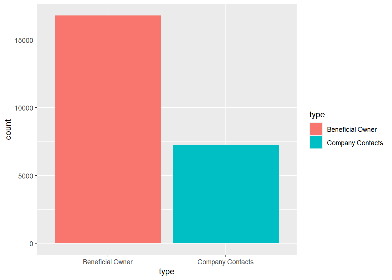
Similarly, we explore the created nodes table. The report above reveals that there are 21515 missing values under “revenue_omu” column and these rows will be subsequently removed when visualising the revenues of the companies. The bar graph comparing the types of entities in the nodes table reveal that there are 3 types of entities - company, company contacts and owners.
skim(mc3_nodes)| Name | mc3_nodes |
| Number of rows | 27622 |
| Number of columns | 5 |
| _______________________ | |
| Column type frequency: | |
| character | 4 |
| numeric | 1 |
| ________________________ | |
| Group variables | None |
Variable type: character
| skim_variable | n_missing | complete_rate | min | max | empty | n_unique | whitespace |
|---|---|---|---|---|---|---|---|
| id | 0 | 1 | 6 | 64 | 0 | 22929 | 0 |
| country | 0 | 1 | 2 | 15 | 0 | 100 | 0 |
| type | 0 | 1 | 7 | 16 | 0 | 3 | 0 |
| product_services | 0 | 1 | 4 | 1737 | 0 | 3244 | 0 |
Variable type: numeric
| skim_variable | n_missing | complete_rate | mean | sd | p0 | p25 | p50 | p75 | p100 | hist |
|---|---|---|---|---|---|---|---|---|---|---|
| revenue_omu | 21515 | 0.22 | 1822155 | 18184433 | 3652.23 | 7676.36 | 16210.68 | 48327.66 | 310612303 | ▇▁▁▁▁ |
ggplot(data = mc3_nodes, aes(x = type, fill = type)) +
  geom_bar()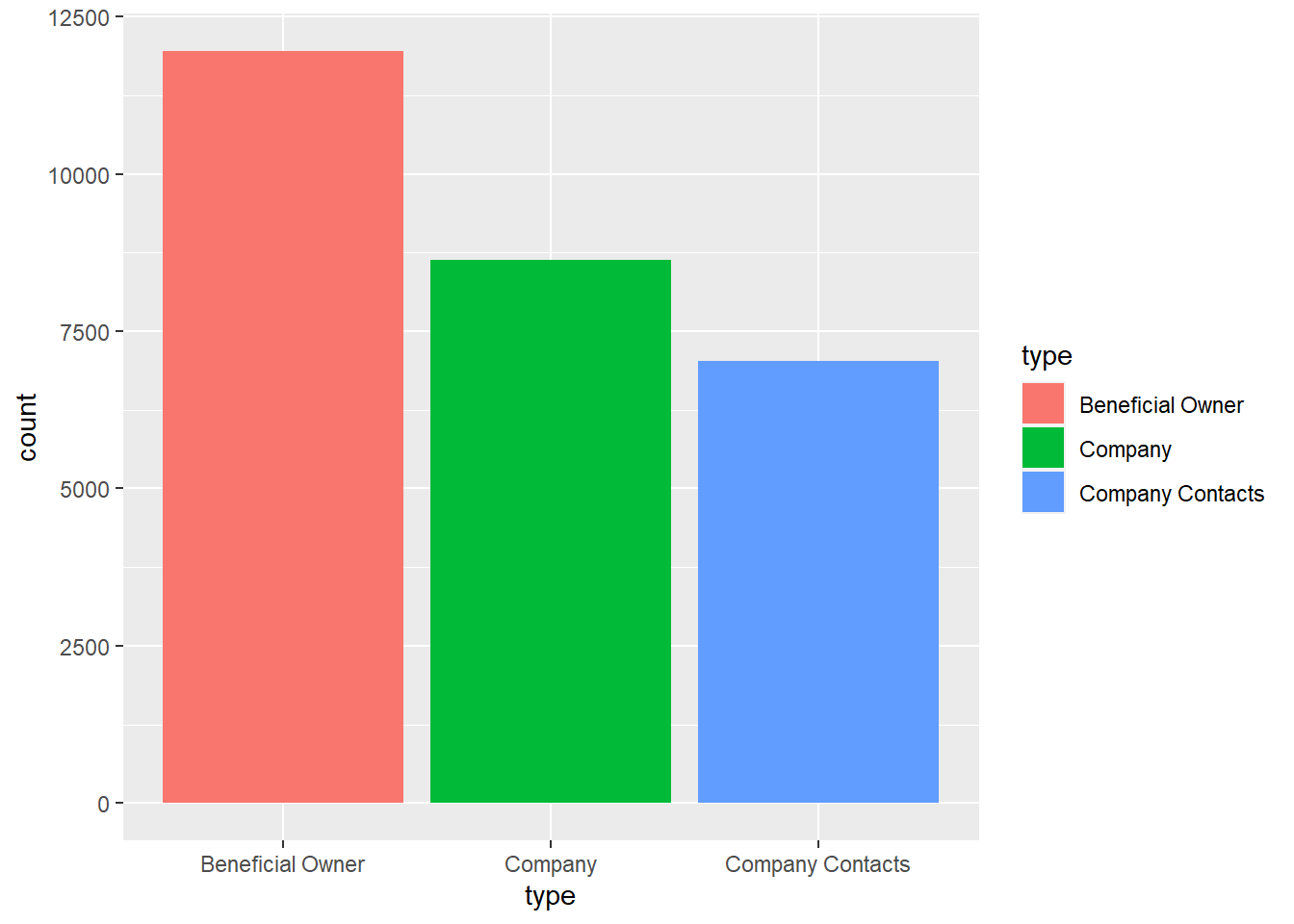
We would need to extract the embedded lists of entities found under the “Source” column in the original edges table, and itemise into individual rows. This is done by splitting the string in the embedded lists into edges sub-table, and removing whitespaces and irrelevant characters.
#Extract lists from the edges table
mc3_edge_unclean <- mc3_edges %>%
filter(substr(source,1,2) %in% "c(")# Break up the lists in the edge file by splitting the string
mc3_edge_broken <- unnest(mc3_edge_unclean, source = strsplit(as.character(source), "\\(|\\,|\\)"))# Remove whitespaces amd filter records with "c" value
#Create edges table incorporating the unlisted values
mc3_edge_broken <- mc3_edge_broken %>%
mutate(source = gsub("\"", "", source)) %>%
filter(source !="c") %>%
mutate(source = trimws(source)) %>%
mutate(target = trimws(target)) %>%
group_by(source, target, type) %>%
summarise(weights = n()) %>%
filter(source != target) %>%
ungroup()From the original edges table, we will remove the lists, and subsequently concatenate the itemised values which were extracted from the embedded lists. This will form the clean edges table.
#Create edges table without embedded lists from original edges table
mc3_edges_without_list <- mc3_edges %>%
  filter(!substr(source,1,2) %in% "c(") %>%
  distinct()

#Combine new edges table with edges table incorporated with the unlisted values, to form a combined edges table.
mc3_edges_combined <- rbind(mc3_edges_without_list, mc3_edge_broken)
Next we will join the edges table with nodes table into combined edge table by mapping edge “source” column in edge table with “id” column in nodes table. This will provide us with the attribute details of the “source” entities in the edges table. Next, we assign “Company” type to the “source” entities on assumption that they are companies. The edges table will be used to derive the data for subsequent visualisation.
mc3_edges_bysource <- left_join(mc3_edges_combined, mc3_nodes,
by = c("source" = "id"))#Assign source type as "Company"
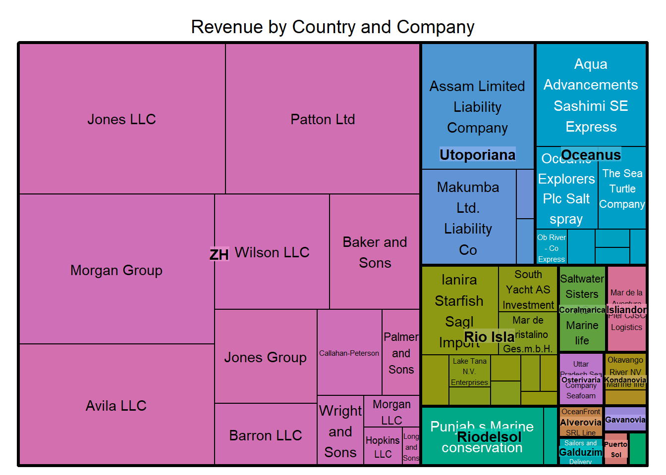
mc3_edges_bysource$type.y <- "Company"The treemap is constructed based on the top 50 companies that generates the highest revenues. It is observed that, of the top 50 companies with the highest revenues, more than half of the total revenues are earned by companies registered in ZH country. The top 3 highest earning companies are Jones LLC, Patton Ltd and Morgan Group. The diagram also revealed that Assam Limited Liability Company and Aqua Advancements Sashimi SE Express are the highest earning company in Utoporiana country and Oceanus country respectively.
#Rename relevant columns as "source type" and "target type"
#Filter combined edge table by removing "unknown" and "character(0)" values under "Product_services" column for subsequent relevant visualisation.
mc3_edges_bysource1 <- mc3_edges_bysource %>%
  group_by(source, target, type.y, type.x, country, weights, revenue_omu, product_services) %>%
  filter(source!=target) %>%
  rename(source_type = type.y) %>%
  rename(target_type = type.x) %>%
  filter(product_services != "Unknown") %>%
  filter(product_services != "character(0)") %>%
ungroup()#Derive new edge table
mc3_edges_toprevenue <- mc3_edges_bysource1 %>%
select (source, source_type, country, weights, revenue_omu, product_services) %>%
group_by(source) %>%
arrange(desc(revenue_omu)) %>%
distinct() %>%
ungroup()#Filter top 50 companies with highest revenues
mc3_edges_toprevenue_filtered <- mc3_edges_toprevenue %>%
filter (source_type == "Company") %>%
slice_max(order_by = revenue_omu, n = 50)#Construct treemap
treemap(mc3_edges_toprevenue_filtered,
index=c("country", "source"),
vSize="revenue_omu",
vColor="revenue_omu",
title="Revenue by Country and Company",
title.legend = "revenue of company"
)
One of the anormalies that we can detect is the number of companies the individual entities own. We can be suspicious of these individuals if they own an exceptionally high number of companies.
In this visualisation on individuals who own more than 5 companies, we observe that the individual who owns the largest number of companies is John Smith (owns a total of 11 companies). This is followed by Micheal Johnson and Jennifer Smith who owns 9 and 8 companies respectively. We can also infer that this group of owners are dominated by the presence of the Smith family.
#Filter individual owners from edge table, and assign target to be source and vice versa
mc3_edges_indivowners <- mc3_edges_bysource %>%
  select (target, source, type.x, weights) %>%
  group_by(target) %>%
  filter(type.x == "Beneficial Owner") %>%
  rename (sc = target) %>%
  rename (tg = source) %>%
  distinct() %>%
ungroup()#Filter individuals who own more 5 companies
mc3_edges_indivowners_filtered <- mc3_edges_indivowners %>%
group_by(sc) %>%
filter(n() > 5) %>%
ungroup()#Create corresponding nodes table out of the edges table
id1_inv <- mc3_edges_indivowners_filtered %>%
select(sc) %>%
rename(id = sc)
id2_inv <- mc3_edges_indivowners_filtered %>%
select(tg) %>%
rename(id = tg)
mc3_nodes_indivowners_filtered <- rbind(id1_inv, id2_inv) %>%
distinct()#prep format for plotting
mc3_edges_indivowners_filtered <- mc3_edges_indivowners_filtered %>%
rename(from = sc) %>%
rename(to = tg) %>%
#filter (target_type == "companies") %>%
filter(from!=to) %>%
ungroup()#Plot interactive graph
visNetwork(mc3_nodes_indivowners_filtered, mc3_edges_indivowners_filtered) %>%
visNodes(color = list(background = "pink", border = "red")) %>%
visEdges(arrows = "to") %>%
visIgraphLayout(layout = "layout_with_gem") %>%
visOptions(highlightNearest = TRUE, nodesIdSelection = TRUE) %>%
visLegend() %>%
visLayout(randomSeed = 123)While it is true that companies are typically registered in the country where they are headquartered or where they conduct their primary operations, it is not unheard of for companies to be registered in multiple countries. Nevertheless for our visualisation, we wish to identify such companies as such situations may not be entirely normal and these companies may potentially breach some form of legality.
The bar chart below shows the companies that have registered in more than one country. It reveals that Aqua Aura SE marine Life has the highest number of countries it registers in (9 countries in total). This is followed by Transit Limited Liability Company as well as Tamil Nadu S A/S, with both registered in 4 countries each.
#Derive specific edge table and filter all companies
mc3_edges_country <- mc3_edges_bysource %>%
  select (source, country, type.y) %>%
  group_by(source) %>%
  filter(type.y == "Company") %>%
  distinct() %>%
ungroup()#Filter companies that are registered in more than 1 country
mc3_edges_country_filtered_one <- mc3_edges_country %>%
group_by(source) %>%
filter(n() > 1) %>%
ungroup()ggplot(data = mc3_edges_country_filtered_one, aes(x = source)) +
geom_bar(fill = "lightblue") +
coord_flip() +
xlab("Companies") +
ylab("No of countries registered") +
scale_y_continuous(breaks = pretty_breaks(n = 5)) +
theme(axis.text.y = element_text(size = 4))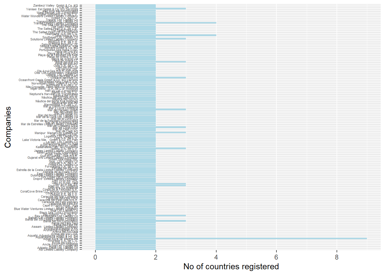
To gather deeper insights, we will drill down to more extreme cases to uncover deeper insights on such companies. The visualisation below focuses on companies which are registered in more than 2 countries. From the network plot, we can pick up the names of the countries that companies register in. In the case of Aqua Aura SE Marine Life, this company has registered in the 9 countries - Oceanus, Coralmarica, Alverossia, Nalakond, Rio Isla, Talandria, Icarnia, Mawazam and Isliandor.
#Filter companies that are registered in more than 2 countries
mc3_edges_country_filtered <- mc3_edges_country %>%
  group_by(source) %>%
  filter(n() > 2) %>%
ungroup()#Create corresponding nodes table out of the edges table
id1_con <- mc3_edges_country_filtered %>%
select(source) %>%
rename(id = source)
id2_con <- mc3_edges_country_filtered %>%
select(country) %>%
rename(id = country)
mc3_nodes_country_filtered <- rbind(id1_con, id2_con) %>%
distinct()#prep format for plotting
mc3_edges_country_filtered <- mc3_edges_country_filtered %>%
rename(from = source) %>%
rename(to = country) %>%
filter(from!=to) %>%
ungroup()#Plot interactive graph
visNetwork(mc3_nodes_country_filtered, mc3_edges_country_filtered) %>%
visNodes(color = list(background = "lightgreen", border = "orange")) %>%
visEdges(arrows = "from") %>%
visIgraphLayout(layout = "layout_with_gem") %>%
visOptions(highlightNearest = TRUE, nodesIdSelection = TRUE) %>%
visLegend() %>%
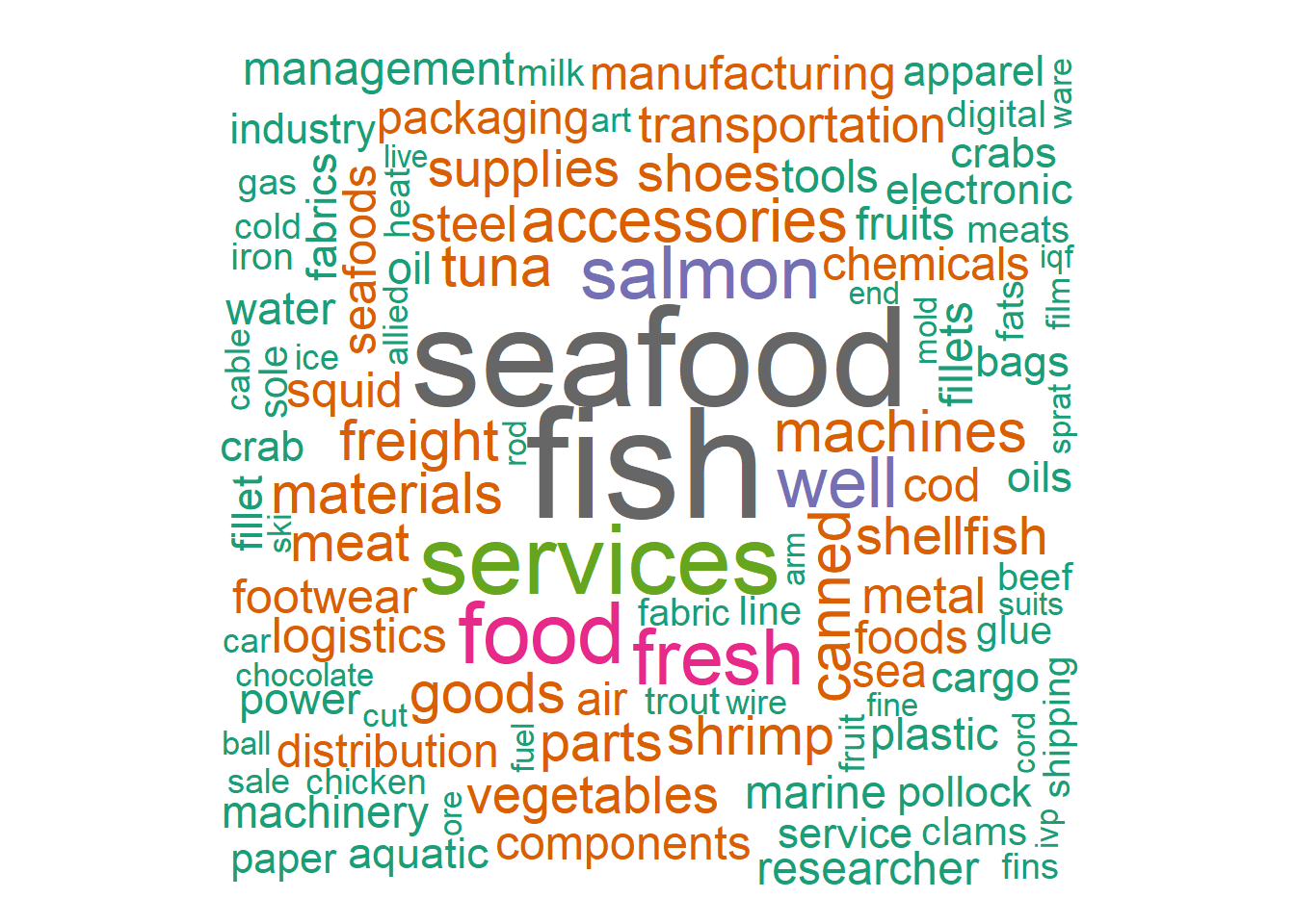
visLayout(randomSeed = 123)The word cloud provides an overview of the range of product services provided by the companies. It also provides us with an indication of the more common business groups and the product mix. We can infer that most of the companies are dealing in food related services, in particular seafood and fish. In terms of the fish types, the salmon would seem to be the most common.
column_values <- mc3_edges_toprevenue$product_services#Create a Corpus
corpus <- Corpus(VectorSource(column_values))
#Preprocess the words
corpus <- tm_map(corpus, content_transformer(tolower))
corpus <- tm_map(corpus, removePunctuation)
corpus <- tm_map(corpus, removeNumbers)
#Add custom stopwords
custom_stopwords <- c("products", "systems", "including", "solutions", "industrial", "wide", "short", "fat", "die", "related", "equipment", "range", "offers", "kits", "frozen", "wild", "kit", "soft", "hard", "non", "cooked", "ltl", "dust", "full", "processing", "high", "dried", "far", "low", "roll", "flat", "raw", "source", "lcl", "men", "strip", "include", "multi", "natural", "general", "unit", "care", "hot", "rare", "dry", "set", "provides", "involved", "ends", "chum", "freelance", "hvac", "etc")
corpus <- tm_map(corpus, removeWords, stopwords("english"))
corpus <- tm_map(corpus, removeWords, custom_stopwords)
#Create a term document matrix
tdm <- TermDocumentMatrix(corpus)
#Convert the term document matrix to a matrix
m <- as.matrix(tdm)
#Calculate word frequencies
word_freq <- sort(rowSums(m), decreasing = TRUE)
#Create the word cloud
wordcloud(words = names(word_freq), freq = word_freq, scale = c(5, 1), random.order = FALSE, colors = brewer.pal(8, "Dark2"))